③ 根轨迹的渐近线:\(\sigma_a=\dfrac{-2.61-25-997.39}{4}=-256.25\),\(\varphi_a=\pm\dfrac{\pi}{4},\pm\dfrac{3\pi}{4}\)。
④ 根轨迹的分离点:根轨迹的分离点坐标满足
\[\frac{1}{d}+\frac{1}{d+2.61}+\frac{1}{d+25}+\frac{1}{d+997.39}=0\]
解得 \(d_1=-750\),\(d_2=-1.27\)
由于闭环主导极点的阻尼比为 \(\zeta=0.5\),则可设闭环主导极点为 \(s=-\sigma+j(1.732\sigma)\)。
由闭环根轨迹的相角条件可得
\[\theta_{sp_1}+\theta_{sp_2}+\theta_{sp_3}+\theta_{sp_4}=180°\]
又
\[\theta_{sp_1}=120°,\quad \theta_{sp_2}=\arctan[(2.61-\sigma)/1.732\sigma]\]
\[\theta_{sp_3}=\arctan[(25-\sigma)/1.732\sigma],\quad \theta_{sp_4}\approx0\]
故可解得 \(\sigma=1.13\)
即闭环主导极点为 \(s=-1.13+j1.96\)
根据以上几点,其概略根轨迹图如图4-133所示。
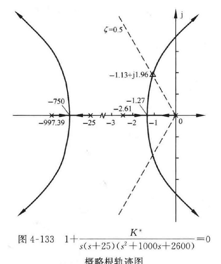
对应的 \(K^*\) 值可由根轨迹的幅值条件求得
\[K^*=|s-p_1|\times|s-p_2|\times|s-p_3|\times|s-p_4|=1.33\times10^5\]
仿真曲线如图4-134、图4-135所示。
MATLAB 程序:exe439.m
G=zpk([],[0 -25 -2.61 -997.39],1);
figure,  rlocus(G); axis([-1000 -20 -750 750]);          %根轨迹左半部分
figure,  rlocus(G); axis([-5 5 -20 20]);                 %根轨迹右半部分
figure,  rlocus(G); z=0.5;   sgrid(z,'new'); axis([-4 2 -5 5]);  %确定主导极点
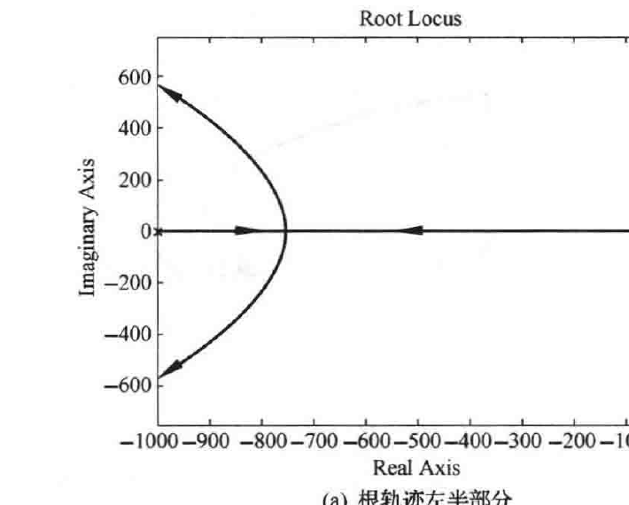
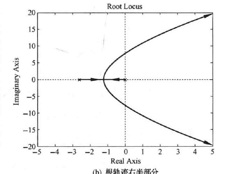
图4-134 \(1+\dfrac{K^*}{s(s+25)(s^2+1000s+2600)}=0\) 根轨迹图(MATLAB)
(页码:· 206 ·)