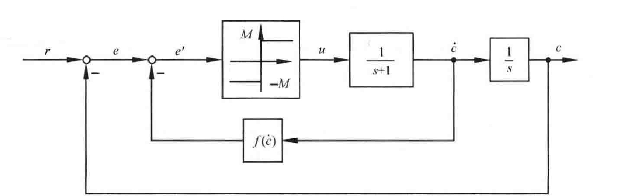
图 8-61　非线性系统结构图

解　(1) 绘制相轨迹。因为在比较点处有 \(e=r-c=1-c,\ \dot{e}=-\dot{c}\)，所以令 \(f(\dot{c})=\beta\)，\(e'=r-c-\beta\dot{c}=e+\beta\dot{e}\)，并根据系统结构图可知 \(\ddot{c}+\dot{c}=u\)，其中 \(u\) 为非线性环节的输出

综合并整理可得系统微分方程为

开关线为 \(e+\beta\dot{e}=0\)。

在 Ⅰ 区 \((e+\beta\dot{e}>0)\)，令 \(\alpha=\dfrac{\mathrm{d}\dot{e}}{\mathrm{d}e}=-\dfrac{M+\dot{e}}{\dot{e}}\) 为相轨迹切线处斜率，得等倾线方程为

在 Ⅱ 区 \((e+\beta\dot{e}<0)\)，令 \(\alpha=\dfrac{\mathrm{d}\dot{e}}{\mathrm{d}e}=-\dfrac{\dot{e}-M}{\dot{e}}\) 为相轨迹切线处斜率，得等倾线方程为

表 8-6 给出了不同 \(\alpha\) 值下等倾线的斜率：

表 8-6　不同 \(\alpha\) 值下等倾线的斜率

若 \(M=1,f(\dot{c})=0,r(t)=1(t)\)，即 \(\beta=0\)，无速度反馈，因此当初始条件 \(e(0)=1,\dot{e}(0)=0\) 时，根据等倾线法和下述 MATLAB 程序可得系统的相平面图和状态曲线分别如图 8-62 和图 8-63 所示。另若 \(M=1,f(\dot{c})=1,r(t)=1(t)\)，即 \(\beta=1\)，初始条件 \(e(0)=1,\dot{e}(0)=0\) 时，根据等倾线法和 MATLAB 程序可得系统的相平面图和状态曲线分别如图 8-64 和图 8-65 所示。

MATLAB 程序：exe824.m

clc;clear
t=0:0.01:10;e0=[1 0]';[t,e]=ode45('sys824',t,e0);
figure(1);plot(e(:,1),e(:,2));grid
figure(2);plot(t,1-e(:,1));grid

调用函数：sys824.m

· 454 ·